Conway's Game of Life on GPU using CUDA
This project compares performance of CPU and GPU in evaluation of famous Conway's Game of Life. The performance was tested on three different implementations. The most sophisticated version of the algorithm on GPU stores data in one bit-per-cell array and leads to a speed-up of 480x compared to the serial CPU algorithm. The best implementation for CPU turned out to be a lookup-table approach leading to 60x speedups over serial CPU. The report contains a detailed explanation of used algorithms, measurements, and code of the whole project for download.
Source code is available on GitHub: NightElfik/Game-of-life-CUDA
1. Introduction#
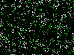
Conway's Game of Life rendered with effect of dying cells. 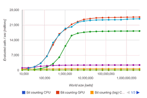
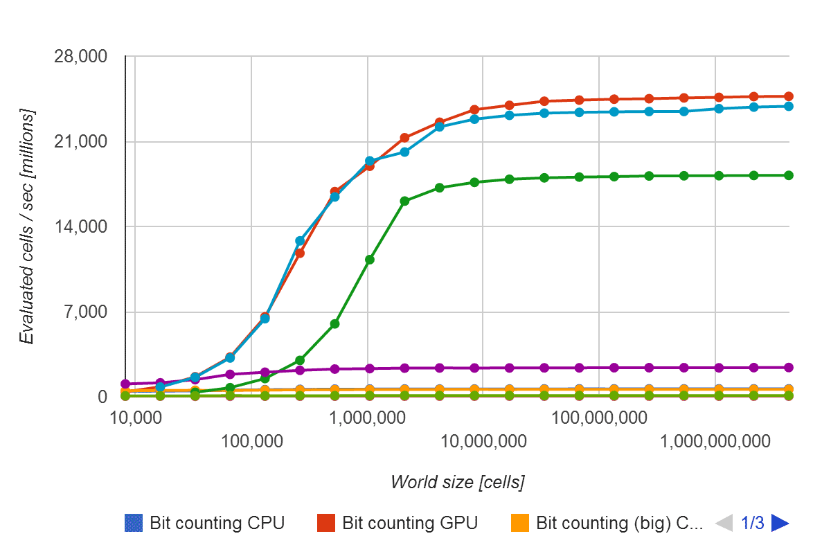
Final evaluation speed. See the Conclusion chapter for details of this graph. 
Interface of the program. 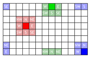
Cyclic world explanation. 
Zoomed-out world (16 cells per pixel).

Conway's Game of Life is a well known cellular automaton which simulates alive and dead cells on an infinite square grid (a world). The word game is quite misleading because only interaction of a human is usually the initial state of the world.
Every cell in the world is either dead or alive. The world evolves in generations also called iterations. The alive state of every cell is determined by the number of living cells around it.
This project was the final assignment in GPU Programming in CUDA (CGT 620) class. The goal of this assignment was to compare a single threaded CPU implementation to a GPU implementation using CUDA. I thought that this comparison is quite unfair for the CPU because it can perform parallel operations as well as GPU so I decided to implement a parallel algorithm for the CPU as well. And on top of that, I implemented two other and faster algorithms on both CPU and GPU that use only one bit per cell and perform life iterations using bit counting and lookup table methods.
All described algorithms in this article were developed by me from scratch — no textbooks or other sources were used. Full source code is available on GitHub.
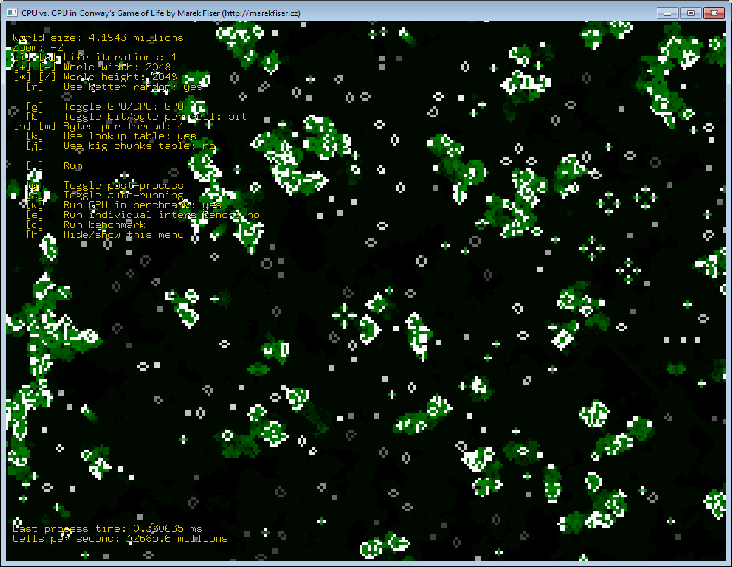
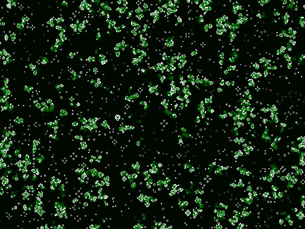 Figure 1: Print-screen of the finished program of Conway's game of life.
Game of Life rules#
Rules of Conway's Game of Life are pretty simple. The world is an infinite square grid where every cell has eight neighbors (Moore neighborhood). Every cell is dead or alive. The world can be visualized as an image with a white pixel for an alive cell and a black pixel for a dead cell (or vice versa).
The life is evolving iteratively. In every iteration, the alive state of every cell is evaluated according to the following rules:
- Any live cell with fewer than two live neighbors dies, as if caused by under-population.
- Any live cell with two or three live neighbors lives on to the next generation.
- Any live cell with more than three live neighbors dies, as if by overcrowding.
- Any dead cell with exactly three live neighbors becomes a live cell, as if by reproduction.
The rules can be observed on evolving patterns in Figure 2.

The Beehive is still - doesn't change as it evolves. (from Wikipedia). 
The Blinker has a period of two iterations. (JokeySmurf from Wikipedia). 
The Glider pattern moving over time. (RodrigoCamargo from Wikipedia).
The rules can be simplified to the alive condition shown in Code listing 1. In words, a cell is born (or stays alive) if it has exactly three alive neighbors or if it has two alive neighbors and it is alive as well. Otherwise it dies (or stays dead).
1
2
3
4
5
6
if (aliveNeighbors == 3 || (aliveNeighbors == 2 && isCellAlive[x][y])) {
	isCellAlive[x][y] = true;
}
else {
	isCellAlive[x][y] = false;
}
Any condition in the form if (...condition...) { x = true; } else { x = false; } can be simplified and inlined to x = ...condition...; so Code listing 2 shows the inlined alive condition.
1
isCellAlive[x][y] = aliveNeighbors == 3 || (aliveNeighbors == 2 && isCellAlive[x][y]));
Cyclic world#
By definition, the life world is infinite. Unfortunately, computers are not very good at representing infinite data structures so world size has to be limited. There are some clever ways how to represent very, very big worlds that seem infinite but this is not the direction I want to go.
The simplest way how to make a world infinite is to make it cyclic. This means that the left neighbor of the leftmost column is the rightmost column and vice versa. This makes the world infinite in terms that you can go any direction as far as you want without hitting any edge. Of course that the total number of cells in a cyclic world is finite and the infinity is not real, but good enough for Game of Life purposes. An example of cells and their neighborhood in a cyclic world is shown in Figure 3.
The actual implementation of a cyclic world is done by using the modulus operator.
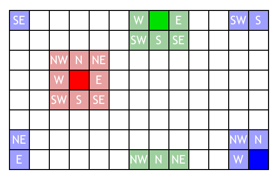 Figure 3: Red, green, and blue cells with their Moore neighborhood in a cyclic world.
2. Basic implementation#
In theory, Conway's Game of Life is pretty simple and straightforward to implement. However, one has to be careful with implementation details to achieve good performance.
The first optimization is to get rid of as many if statements as possible.
If statements are not a good friend with CPU and especially not with GPU.
On GPU, the if statement may cause warp divergence that slows down execution.
Counting of neighbors of a cell can be done by using eight if statements but those ifs can be completely avoided.
An integer like char (I actually used unsigned char or ubyte) can be used for representing alive state of a cell as value 1 or 0 (alive or dead).
This slight change of representation changes the neighbor counting code from eight if statements to seven summations (pseudo-code shown in Code listing 3).
1
2
3
uint aliveCells = isCellAlive[x-1][y-1] + isCellAlive[x][y-1] + isCellAlive[x+1][y-1]
	+ isCellAlive[x-1][y] + isCellAlive[x+1][y]
	+ isCellAlive[x-1][y+1] + isCellAlive[x][y+1] + isCellAlive[x+1][y+1];
The second optimization is to use a single array instead of an array of arrays.
This makes the code less readable but more effective.
Every cell access code will change from isCellAlive[x][y] to isCellAlive[y * width + x].
1
2
3
4
5
6
7
// Y-coordinates y0, y1 and y2 are already pre-multiplied with world width.
inline ubyte countAliveCells(size_t x0, size_t x1, size_t x2,
		size_t y0, size_t y1, size_t y2) {
	return m_data[x0 + y0] + m_data[x1 + y0] + m_data[x2 + y0]
		+ m_data[x0 + y1] + m_data[x2 + y1]
		+ m_data[x0 + y2] + m_data[x1 + y2] + m_data[x2 + y2];
}
Serial CPU implementation#
The actual serial implementation of Conway's Game of Life on the CPU is shown in Code listing 5.
The method aliveCells is shown in Code listing 4.
The method computeIterationSerial computes one iteration of Conway's Game of Life in the array m_data using m_resultData as a helper array.
Two arrays are necessary to avoid errors in computation caused by overriding cell states.
The source and result arrays are swapped at the end so the result will be stored in m_data.
1
2
3
4
5
6
7
8
9
10
11
12
13
14
15
16
17
18
19
20
21
22
23
24
25
26
typedef unsigned char ubyte;

ubyte* m_data;
ubyte* m_resultData;

size_t m_worldWidth;
size_t m_worldHeight;
size_t m_dataLength;  // m_worldWidth * m_worldHeight

void computeIterationSerial() {
	for (size_t y = 0; y < m_worldHeight; ++y) {
		size_t y0 = ((y + m_worldHeight - 1) % m_worldHeight) * m_worldWidth;
		size_t y1 = y * m_worldWidth;
		size_t y2 = ((y + 1) % m_worldHeight) * m_worldWidth;

		for (size_t x = 0; x < m_worldWidth; ++x) {
			size_t x0 = (x + m_worldWidth - 1) % m_worldWidth;
			size_t x2 = (x + 1) % m_worldWidth;

			ubyte aliveCells = countAliveCells(x0, x, x2, y0, y1, y2);
			m_resultData[y1 + x] =
				aliveCells == 3 || (aliveCells == 2 && m_data[x + y1]) ? 1 : 0;
		}
	}
	std::swap(m_data, m_resultData);
}
Parallel CPU implementation#
Conway's Game of Life can be parallelized very easily since every cell needs only information about its neighbors. The parallel code in Code listing 6 is nearly identical to the serial code. The only difference is the replacement of the serial for-cycle with a parallel one.
The Concurrency::parallel_for is a feature from the standard Microsoft library that can be found in header ppl.h (Parallel Patterns Library).
This library makes parallel programming so much easier and closer to C# (a language which I know the best).
Just in case anybody is wondering how Concurrency::parallel_for works, it gets a starting index, an end index, an increment,
and a reference to a function (or lambda function) which will be called for every index in the range but in parallel.
The function automatically uses the maximum number of available hardware cores on the current machine.
If a machine has only one processor with one core and no hyper-threading, the code will be actually serial.
You may be wondering if usage of a static function could be faster than construction of the lambda function on every invocation. I was wondering too. The measurements shown in Figure 4 in the next section reveal that there is no significant difference between those two approaches. Actually, the lambda function is sometimes a bit faster, but that was probably just some noise.
1
2
3
4
5
6
7
8
9
10
11
12
13
14
15
16
17
18
19
20
21
22
23
24
25
26
typedef unsigned char ubyte;

ubyte* m_data;
ubyte* m_resultData;

size_t m_worldWidth;
size_t m_worldHeight;
size_t m_dataLength;  // m_worldWidth * m_worldHeight

void computeIterationParallel() {
	auto evaluateCell = [&] (size_t index) {
		size_t x1 = index % m_worldWidth;
		size_t y1 = index - x1;
		size_t y0 = (y1 + m_dataLength - m_worldWidth) % m_dataLength;
		size_t y2 = (y1 + m_worldWidth) % m_dataLength;
		size_t x0 = (x1 + m_worldWidth - 1) % m_worldWidth;
		size_t x2 = (x1 + 1) % m_worldWidth;

		ubyte aliveCells = countAliveCells(x0, x1, x2, y0, y1, y2);
		m_resultData[y1 + x1] =
			aliveCells == 3 || (aliveCells == 2 && m_data[x1 + y1]) ? 1 : 0;
	};

	Concurrency::parallel_for<size_t>(0, m_worldWidth * m_worldHeight, 1, evaluateCell);
	std::swap(m_data, m_resultData);
}
CPU performance evaluation#
Just for curiosity, I compared performance of serial and parallel CPU implementations. My CPU is Intel Xeon E5530 @ 2.40GHz with 4 cores (8 threads). I was hoping that the parallel implementation will be more than 4 times faster since my machine has 4 physical cores and 8 threads.
The performance was measured on the world that contained from 213 (8 thousand) to 232 (4 billion) cells. The reported values are medians from five independent measurements. 16 iterations of life were performed in every measurement and total time was divided by 16 to get an average time per iteration. The results of the CPU benchmark are shown in Figure 4 and as you can see the parallel implementation is roughly two times faster.
I was quite surprised that the speedup was even less than three times. Low speedup is probably caused by low memory throughput since the code does a lot of memory I/O and not too many arithmetic operations.
You can also see a little bit different speedups for the static function versus the lambda function. I am not very sure what is causing the difference, however, for larger worlds, the static function is slightly faster.
Simple GPU implementation#
All GPU implementations described in this article use the CUDA technology. It is not the only technology for using GPUs for general computing, others are for example OpenCL or DirectCompute. However, this project was made for a CUDA class so the choice of technology was easy.
The simple GPU implementation is very similar to the parallel CPU implementation. The only significant difference is the added for-cycle in the CUDA kernel. This cycle ensures that if the kernel is invoked with less threads than necessary, every thread will loop through more cells to compute all of them. Since the number of cells can go easily to very high numbers (billions), this approach is necessary. Code listing 7 shows the CUDA kernel.
The code that allocates and copies memory from the CPU to GPU is not shown here because there is nothing special,
just cudaMalloc, cudaMemcpy and cudaFree.
Well, actually cudaMalloc and cudaFree are called only when the size of the world changes.
This avoids unnecessary allocating, deallocating and copying of memory.
1
2
3
4
5
6
7
8
9
10
11
12
13
14
15
16
17
18
19
20
21
22
__global__ void simpleLifeKernel(const ubyte* lifeData, uint worldWidth,
		uint worldHeight, ubyte* resultLifeData) {
	uint worldSize = worldWidth * worldHeight;

	for (uint cellId = __mul24(blockIdx.x, blockDim.x) + threadIdx.x;
			cellId < worldSize;
			cellId += blockDim.x * gridDim.x) {
		uint x = cellId % worldWidth;
		uint yAbs = cellId - x;
		uint xLeft = (x + worldWidth - 1) % worldWidth;
		uint xRight = (x + 1) % worldWidth;
		uint yAbsUp = (yAbs + worldSize - worldWidth) % worldSize;
		uint yAbsDown = (yAbs + worldWidth) % worldSize;

		uint aliveCells = lifeData[xLeft + yAbsUp] + lifeData[x + yAbsUp]
			+ lifeData[xRight + yAbsUp] + lifeData[xLeft + yAbs] + lifeData[xRight + yAbs]
			+ lifeData[xLeft + yAbsDown] + lifeData[x + yAbsDown] + lifeData[xRight + yAbsDown];

		resultLifeData[x + yAbs] =
			aliveCells == 3 || (aliveCells == 2 && lifeData[x + yAbs]) ? 1 : 0;
	}
}
Code listing 8 shows the code for kernel invocation.
Notice the usage of the same trick with std::swap that is used in the CPU implementation,
two buffers are allocated and they are swapped between iterations.
This means that there is no memory copying of data between the CPU and GPU between consecutive iterations.
The number of threads per block is a parameter because I will run more experiments with different settings of threads per block to see what configuration performs the best.
1
2
3
4
5
6
7
8
9
10
11
12
void runSimpleLifeKernel(ubyte*& d_lifeData, ubyte*& d_lifeDataBuffer, size_t worldWidth,
		size_t worldHeight, size_t iterationsCount, ushort threadsCount) {
	assert((worldWidth * worldHeight) % threadsCount == 0);
	size_t reqBlocksCount = (worldWidth * worldHeight) / threadsCount;
	ushort blocksCount = (ushort)std::min((size_t)32768, reqBlocksCount);

	for (size_t i = 0; i < iterationsCount; ++i) {
		simpleLifeKernel<<<blocksCount, threadsCount>>>(d_lifeData, worldWidth,
			worldHeight, d_lifeDataBuffer);
		std::swap(d_lifeData, d_lifeDataBuffer);
	}
}
GPU performance evaluation#
The CUDA kernel can be invoked with different settings of threads per block (tpb). Different values result in significantly different performance. Performance analysis shown in Figure 5 was run to determine the best value. Reported times are medians from 15 runs. For 32 threads per block, the GPU is not saturated and the performance is not the best. All other settings are quite comparable.
The GPU that was used for all benchmarks is GeForce GTX 580 with 1.5 GB of graphics memory and 512 CUDA cores. Comparison with the CPU is in the following section.
CPU vs. GPU#
The final performance comparison of the basic life evaluation algorithm is shown in Figure 6. The comparison is presented as a speedup over the serial CPU implementation because the serial CPU is very stable at 50 million evaluated cells per second.
As you can see in Figure 6, the GPU is significantly faster than the CPU. The speedup of the GPU algorithm over the serial CPU algorithm is reaching 143x compared to the speedup of the parallel CPU that is just 2x.
The evaluation of the cells is very heavy on memory I/O and not so much on arithmetic operations. The superiority of the GPU comes from its very fast memory chips with much higher memory throughput than CPU's RAM. Note that the reported speedup of the GPU is over the serial CPU implementation, the speedup over the parallel CPU implementation is about 70x.
The next chapter talks about an improved algorithm that reaches even higher speedups for both CPU and GPU implementations.
3. Advanced implementation: 1 bit per cell#
I was quite satisfied with 140x speedup of the basic GPU implementation over the serial CPU but I decided to boost GPU's ego even further by a hopefully faster implementation. Actually – two implementations. This chapter explains an easier one, next section 4: Advanced implementation: lookup table talks about a more complicated one.
Every life cell has two states (alive or dead) which were so far represented as integers 1 and 0. I asked myself a question:
Why waste a whole 8-bit number to encode just 0's and 1's?
Usage of 1 bit per cell could be potentially more efficient and it could also cut memory requirements 8-times.
So how to speed up cell state evaluation?
The obvious way is to get rid of the summing part that is slow because it has too many memory reads,
8 memory reads per cell to be exact.
If a life cell were stored in one bit, a single read of a byte would actually read 8 cells.
Even further, a single read of unsigned int (uint) retrieves 32 cells at once.
The idea of a bit per cell sounds promising, but there is a little catch.
Cells in one uint are in a row, but an area of 3x3 cells is needed in order to evaluate a single cell.
This means that three rows are needed, but it is still better than 9 memory reads.
Evaluation of the cells#
The goal is to evaluate a whole byte of data (8 cells). It is necessary to load three rows and then it is possible to evaluate the middle row cell by cell by counting the number of living cells. The problem is that the neighborhood area overlaps to bytes before and after the current block as shown in Figure 7. This adds quite large overhead. Instead of reading 3 bytes and evaluating 1 byte, 9 bytes need to be read.
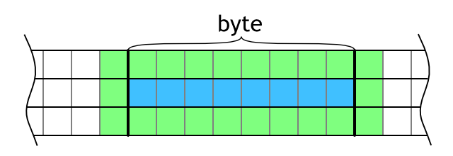 Figure 7: Evaluation of a byte of data (blue area) needs cells from neighboring bytes (green area).
This overhead can be significantly reduced by evaluating more consecutive blocks in the row as shown in Figure 8. Actually, the overhead is constant (2×3 bytes) no matter how many blocks are evaluated in between them. This means that the more bytes evaluated in the row, the better. However, more blocks in the row means more work per thread and too much work per thread can stall the GPU which is not good.
It is hard to guess what is the magical number of consecutive processed blocks (bytes) that would result in the best performance; I will leave this as a parameter of the method.
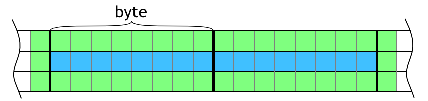 Figure 8: Visualization of overlapping neighboring cells on the left and right.
Blue area shows evaluated cells and green area highlights neighbors that are necessary for evaluation.
Figure 8: Visualization of overlapping neighboring cells on the left and right.
Blue area shows evaluated cells and green area highlights neighbors that are necessary for evaluation.GPU implementation#
Code listing 9 shows the CUDA kernel. It is quite lengthy but I will try to describe it in detail in the following paragraphs.
The kernel starts with a scary-looking for-cycle. This cycle ensures that if the kernel is invoked with less threads than cells to process, every thread will loop through more cells to compute all of them.
The first thing computed in the main cycle is x and y coordinates based on given cell ID. All y coordinates are pre-multiplied with data width to avoid unnecessary multiplications later. This is necessary since the data are stored in a 1D array and every y index has to skip a whole row (data width).
Then, variables called data0, data1, and data2 are initialized with the first two bytes of data.
Those 4-byte (32-bit) integer variables represent rows of data and they are used to store three consecutive bytes of data to allow easy evaluation of the middle byte.
Next follows the for-cycle that goes over consecutively evaluated bytes.
This concept was explained in the previous section Evaluation of the cells.
At the beginning of the cycle,
a new byte is pushed to the datan variables by left-shifting existing content by 8 and or-ing new byte.
Then, another cycle goes over 8 cells that are evaluated. At every position, the number of living cells is counted by some (clever) bit operations and based on the sum the result bit is written. Feel free to grab a piece of paper and sketch the bit operations to see what is happening. Basically, it is parallel bit summing on two positions and then summing to the final number.
1
2
3
4
5
6
7
8
9
10
11
12
13
14
15
16
17
18
19
20
21
22
23
24
25
26
27
28
29
30
31
32
33
34
35
36
37
38
39
40
41
42
43
44
45
46
47
48
49
50
__global__ void bitLifeKernelNoLookup(const ubyte* lifeData, uint worldDataWidth,
		uint worldHeight, uint bytesPerThread, ubyte* resultLifeData) {

	uint worldSize = (worldDataWidth * worldHeight);

	for (uint cellId = (__mul24(blockIdx.x, blockDim.x) + threadIdx.x) * bytesPerThread;
			cellId < worldSize;
			cellId += blockDim.x * gridDim.x * bytesPerThread) {

		uint x = (cellId + worldDataWidth - 1) % worldDataWidth;  // Start at block x - 1.
		uint yAbs = (cellId / worldDataWidth) * worldDataWidth;
		uint yAbsUp = (yAbs + worldSize - worldDataWidth) % worldSize;
		uint yAbsDown = (yAbs + worldDataWidth) % worldSize;

		// Initialize data with previous byte and current byte.
		uint data0 = (uint)lifeData[x + yAbsUp] << 16;
		uint data1 = (uint)lifeData[x + yAbs] << 16;
		uint data2 = (uint)lifeData[x + yAbsDown] << 16;

		x = (x + 1) % worldDataWidth;
		data0 |= (uint)lifeData[x + yAbsUp] << 8;
		data1 |= (uint)lifeData[x + yAbs] << 8;
		data2 |= (uint)lifeData[x + yAbsDown] << 8;

		for (uint i = 0; i < bytesPerThread; ++i) {
			uint oldX = x;  // old x is referring to current center cell
			x = (x + 1) % worldDataWidth;
			data0 |= (uint)lifeData[x + yAbsUp];
			data1 |= (uint)lifeData[x + yAbs];
			data2 |= (uint)lifeData[x + yAbsDown];

			uint result = 0;
			for (uint j = 0; j < 8; ++j) {
				uint aliveCells = (data0 & 0x14000) + (data1 & 0x14000) + (data2 & 0x14000);
				aliveCells >>= 14;
				aliveCells = (aliveCells & 0x3) + (aliveCells >> 2)
					+ ((data0 >> 15) & 0x1u) + ((data2 >> 15) & 0x1u);

				result = result << 1
					| (aliveCells == 3 || (aliveCells == 2 && (data1 & 0x8000u)) ? 1u : 0u);

				data0 <<= 1;
				data1 <<= 1;
				data2 <<= 1;
			}

			resultLifeData[oldX + yAbs] = result;
		}
	}
}
CPU implementation and performance evaluation#
A CPU implementation of the bit counting algorithm is nearly identical to the GPU implementation. The implementation is parallel and I did not even investigate a serial version of it. If you are interested in actual implementation details please see the code on GitHub.
The performance of the CPU version was evaluated for a wide range of consecutive evaluated blocks (cb). The evaluation speeds are shown in Figure 9. The basic serial and parallel algorithms are shown in the figure for comparison.
Figure 9 clearly shows that the bit-per-cell algorithm is much faster than the basic one not only saving memory but speeding up the evaluation as well. As expected, the more consecutive evaluated blocks (cb) the better. This is not the case for GPU as you can see in the next section.
GPU performance evaluation#
GPU performance charts are a little harder to produce because there are two parameters that could vary: number of consecutive evaluated blocks and threads per CUDA block. The benchmark was run for all combinations of those two parameters. The best for each of them was reported.
The best performance among threads per CUDA block was for value 128. Figure 10 shows evaluation speeds for different values of consecutive evaluated blocks (cb) compared to the basic GPU implementation described in section 2: Basic implementation. For most values of cb the evaluation speed is higher than the basic GPU implementation. However, the trend that more cb results in better performance as observed in the CPU implementation is not true now. The best value of cb is probably 8, for higher values the performance decreases and for 128 cb the evaluation speed is even lower than for the basic implementation.
For the completeness of the GPU implementation performance evaluation, Figure 11 shows the evaluation speed for different values of threads per CUDA block (tpb). The variance in results is not that big, the only outlier is the lowest value 32 tpb.
This chart nicely shows the speedup of the bit counting implementation over the basic GPU implementation which is about 2.5×. That is more than the speedup for the CPU implementation which was about 2×.
The next section compares the performance of the best performing settings of the CPU and GPU algorithms.
CPU vs. GPU#
For the final comparison of this chapter, the best performing settings were selected for the CPU and GPU. The CPU algorithm performed the best for 128 consecutive evaluated blocks (cb) and the GPU algorithm for 8 cb and 128 threads per CUDA block (tpb). Figure 12 shows speedup of those two measurements and compares them with the basic parallel CPU and basic GPU for 128 tpb.
It is nicely visible that even the improved bit-per-cell CPU implementation is way slower than the basic GPU implementation. The improved GPU implementation is reaching speedups up to 480× over the basic serial CPU implementation.
Optimized memory access#
But I will not stop here. As suggested in the introduction of this chapter, reading of larger memory blocks might be more effective. Most hardware is optimized to read larger memory blocks as opposed to small ones. The idea is to read and write 32-bit words instead of 8-bit bytes.
The implementation has to be substantially changed in order to achieve this improvement. First, three consecutive blocks cannot be accumulated in one variable anymore.
Second, the CPU and GPU are using little endian for representing longer words than a byte. However, little endian stores the bytes in reversed order and it is not possible to process them sequentially. This problem is solved by swapping endianness while reading and writing.
The GPU implementation is shown in Code listing 10 and it is much longer than the previous implementation. This is mainly due to overlaps that are handled separately to save memory and computations.
The implementation on CPU is again very similar to the CUDA kernel and uses Concurrency::parallel_for for parallelization.
1
2
3
4
5
6
7
8
9
10
11
12
13
14
15
16
17
18
19
20
21
22
23
24
25
26
27
28
29
30
31
32
33
34
35
36
37
38
39
40
41
42
43
44
45
46
47
48
49
50
51
52
53
54
55
56
57
58
59
60
61
62
63
64
65
66
67
68
69
70
71
72
73
74
75
__global__ void bitLifeCountingBigChunks(const uint* lifeData, uint worldDataWidth,
		uint worldHeight, uint chunksPerThread, uint* resultLifeData) {

	uint worldSize = (worldDataWidth * worldHeight);

	for (uint cellId = (__mul24(blockIdx.x, blockDim.x) + threadIdx.x) * chunksPerThread;
			cellId < worldSize;
			cellId += blockDim.x * gridDim.x * chunksPerThread) {

		uint x = (cellId + worldDataWidth - 1) % worldDataWidth;  // Start at block x - 1.
		uint yAbs = (cellId / worldDataWidth) * worldDataWidth;
		uint yAbsUp = (yAbs + worldSize - worldDataWidth) % worldSize;
		uint yAbsDown = (yAbs + worldDataWidth) % worldSize;

		uint currData0 = swapEndianessUint32(lifeData[x + yAbsUp]);
		uint currData1 = swapEndianessUint32(lifeData[x + yAbs]);
		uint currData2 = swapEndianessUint32(lifeData[x + yAbsDown]);

		x = (x + 1) % worldDataWidth;
		uint nextData0 = swapEndianessUint32(lifeData[x + yAbsUp]);
		uint nextData1 = swapEndianessUint32(lifeData[x + yAbs]);
		uint nextData2 = swapEndianessUint32(lifeData[x + yAbsDown]);

		for (uint i = 0; i < chunksPerThread; ++i) {
			// Evaluate front overlapping cell.
			uint aliveCells = (currData0 & 0x1u) + (currData1 & 0x1u) + (currData2 & 0x1u)
				+ (nextData0 >> 31) + (nextData2 >> 31)  // Do not count middle cell.
				+ ((nextData0 >> 30) & 0x1u) + ((nextData1 >> 15) & 0x1u)
				+ ((nextData2 >> 16) & 0x1u);

			// 31-st bit.
			uint result = (aliveCells == 3 || (aliveCells == 2 && (nextData1 >> 31)))
				? (1u << 31) : 0u;

			uint oldX = x;  // Old x is referring to current center cell.
			x = (x + 1) % worldDataWidth;
			currData0 = nextData0;
			currData1 = nextData1;
			currData2 = nextData2;

			nextData0 = swapEndianessUint32(lifeData[x + yAbsUp]);
			nextData1 = swapEndianessUint32(lifeData[x + yAbs]);
			nextData2 = swapEndianessUint32(lifeData[x + yAbsDown]);

			// Evaluate back overlapping cell.
			aliveCells = ((currData0 >> 1) & 0x1u) + ((currData1 >> 1) & 0x1u)
				+ ((currData2 >> 1) & 0x1u)
				+ (currData0 & 0x1u) + (currData2 & 0x1u)  // Do not count middle cell.
				+ (nextData0 >> 31) + (nextData1 >> 31) + (nextData2 >> 31);

			// 0-th bit.
			result |= (aliveCells == 3 || (aliveCells == 2 && (currData1 & 0x1u))) ? 1u : 0u;

			// The middle cells with no overlap.
			for (uint j = 0; j < 30; ++j) {
				uint shiftedData = currData0 >> j;
				uint aliveCells = (shiftedData & 0x1u) + ((shiftedData >> 1) & 0x1u)
					+ ((shiftedData >> 2) & 0x1u);

				shiftedData = currData2 >> j;
				aliveCells += (shiftedData & 0x1u) + ((shiftedData >> 1) & 0x1u)
					+ ((shiftedData >> 2) & 0x1u);

				shiftedData = currData1 >> j;
				// Do not count middle cell.
				aliveCells += (shiftedData & 0x1u) + ((shiftedData >> 2) & 0x1u);

				result |= (aliveCells == 3 || (aliveCells == 2 && (shiftedData & 0x2))
					? (2u << j) : 0u);
			}

			resultLifeData[oldX + yAbs] = swapEndianessUint32(result);
		}
	}
}
Performance evaluation of optimized memory access#
Long story short, the promise of some speedup did not happen. Figure 13 shows speedup of the bit counting algorithm on big chunks for the CPU over the previous implementation of bit counting on smaller chunks. For any value of cb the speedup is lower than one. The situation is the same for the GPU, no speedup over the previous implementation as shown in Figure 14.
First, I was quite surprised by this result but then I realized that the overhead of reading small chunks is completely negated by caches.
Thanks to these results I realized how crucial the caches actually are.
I think that the lower performance is caused by the overhead of dealing with large chunks (endianness switching, etc.). The algorithm for smaller chunks is actually faster. Thanks, caches!
4. Advanced implementation: lookup table#
The results from the previous section 3: Advanced implementation: 1 bit per cell were very nice, speedups reaching up to 480× over the basic serial CPU implementation. However, I was hoping to reach even higher speedups by implementing a lookup table evaluation. The problem with the bit counting is that it is quite computation heavy. The GPU has to perform more than a hundred arithmetic operations in order to evaluate a single byte of data.
Instead of counting neighbors,
the state of cells could be easily encoded into a number and a lookup table could be used to evaluate it.
The problem is that the size of a potential lookup table is exponential with the size of the state;
2state cells count to be exact.
Finding optimal evaluation area#
A 3×3 area of cells is needed in order to evaluate a single cell. It would take 8 lookups to evaluate a whole byte of data. If two cells were evaluated at once, only four lookups would be needed but a table would have to be constructed for an area of 4×3 cells.
Generally, the bigger block of data is processed at once, the fewer table lookups and the fewer arithmetic operations are needed, but the bigger lookup table, exponentially bigger.
The goal is to compromise between the size of the table and the number of evaluated cells at once.
The shape of the evaluated area also makes a difference. The ratio between the number of evaluated cells and their neighborhood necessary for their evaluation is the best for square-ish shapes. Data are, however, stored in rows, it is much easier to read a row than a column. This is the reason why only considered areas have 3 rows. There might be some benefit of reading more than 3 rows but I did not go that way.
Figure 15 summarizes all the important factors of several cell configurations.
The table nicely shows how larger areas are more effective but they need to have a much larger lookup table. A small lookup table helps the performance because it can fit into the processor's caches, which is extremely important. Reading from caches is much faster than from main memory. All sizes of evaluated cells are powers of two to be able to align them to 8-bit bytes.
I did not have time to write the code for all options and do the performance analysis so I wanted to do an educated guess what would be the best option. I really liked the 3×10 option because that one would allow me to work with whole bytes (result is 8 bits, one byte). However, a 1 GB lookup table is insane, especially for a GPU with a few GBs of available memory.
Long story short, due to many implementation details and lookup table size I decided to use the 6×3 area.
| Size | Eval. cells per step | Eval. steps | Lookup table rows | Lookup table size (optimal) | Lookup table size (byte per row) |
|---|---|---|---|---|---|
| 3×3 | 1 | 8 | 29 = 512 | 29 ∙ 1 b = 64 B | 29 ∙ 8 b = 512 B |
| 4×3 | 2 | 4 | 212 = 4096 | 212 ∙ 2 b = 1 KB | 212 ∙ 8 b = 4 KB |
| 6×3 | 4 | 2 | 218 = 262144 | 218 ∙ 4 b = 128 kB | 218 ∙ 8 b = 256 kB |
| 3×10 | 8 | 1 | 230 ≈ 1 bil | 230 ∙ 8 b = 1 GB | 230 ∙ 8 b = 1 GB |
Lookup table construction#
I decided to use a lookup table for area 6×3 which means that the lookup table has to have 26∙3 = 218 rows.
The values in this table have 4 bits which makes the table 218 ∙ 4 b = 128 kB big.
The optimal sized table has two entries in every byte which makes access complicated.
I decided to use a sub-optimal solution storing every entry in a byte (not in 4 bits) which makes the table twice as big.
The lookup table is computed by the GPU.
Code listing 11 shows the kernel which is invoked on 218 threads (256 threads per block on 1024 blocks).
The computation itself is pretty straightforward. Every table index represents a 6×3 area of cells. The value on that index represents the result state of the 4 middle cells. The kernel computes just that and saves it to given array.
Helper function getCellState serves to get the bit in coordinates x and y in given 6×3 area of given key key
The lookup table is computed only once per program lifetime and it is kept in the GPU memory all the time. The table takes only 256 KB of GPU memory which is negligible. There is no need for analyzing of computation performance or for trying to make the computation faster. The fact that it is implemented using CUDA is already overkill.
1
2
3
4
5
6
7
8
9
10
11
12
13
14
15
16
17
18
19
20
21
22
23
24
25
26
27
28
29
__global__ void precompute6x3EvaluationTableKernel(ubyte* resultEvalTableData) {
	uint tableIndex = __mul24(blockIdx.x, blockDim.x) + threadIdx.x;

	ubyte resultState = 0;
	// For each cell.
	for (uint dx = 0; dx < 4; ++dx) {
		// Count alive neighbors.
		uint aliveCount = 0;
		for (uint x = 0; x < 3; ++x) {
			for (uint y = 0; y < 3; ++y) {
				aliveCount += getCellState(x + dx, y, tableIndex);
			}
		}

		uint centerState = getCellState(1 + dx, 1, tableIndex);
		aliveCount -= centerState;  // Do not count center cell in the sum.

		if (aliveCount == 3 || (aliveCount == 2 && centerState == 1)) {
			resultState |= 1 << (3 - dx);
		}
	}

	resultEvalTableData[tableIndex] = resultState;
}

inline __device__ uint getCellState(uint x, uint y, uint key) {
	uint index = y * 6 + x;
	return (key >> ((3 * 6 - 1) - index)) & 0x1;
}
GPU implementation#
The CUDA kernel for the implementation of the described lookup table evaluation algorithm is shown in Code listing 12. The code is very similar to the previous bit-counting technique described in section 3: Advanced implementation: 1 bit per cell.
The major difference is in the evaluation itself. Instead of a cycle that counts bits, encoding of life state is performed and the lookup table is used for evaluation.
In order to evaluate a whole byte, two lookups are needed. Figure 16 and the following code snippet show the code for encoding the cell states.
1
2
uint lifeStateHi = ((data0 & 0x1F800) << 1) | ((data1 & 0x1F800) >> 5) | ((data2 & 0x1F800) >> 11);
uint lifeStateLo = ((data0 & 0x1F80) << 5) | ((data1 & 0x1F80) >> 1) | ((data2 & 0x1F80) >> 7);
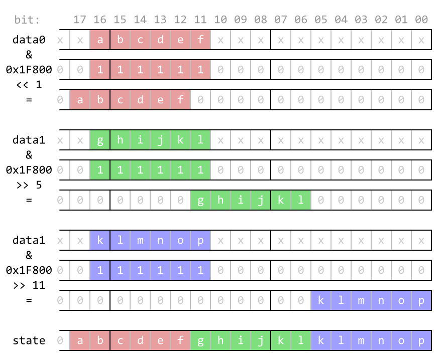 Figure 16: Visualization of encoding of a 6×3 block of data to a single 18-bit number.
The evaluation using a lookup table is as simple as the last line in Code listing 12.
1
2
3
4
5
6
7
8
9
10
11
12
13
14
15
16
17
18
19
20
21
22
23
24
25
26
27
28
29
30
31
32
33
34
35
36
37
38
__global__ void bitLifeKernel(const ubyte* lifeData, uint worldDataWidth,
		uint worldHeight, uint bytesPerThread, const ubyte* evalTableData,
		ubyte* resultLifeData) {
	uint worldSize = (worldDataWidth * worldHeight);

	for (uint cellId = (__mul24(blockIdx.x, blockDim.x) + threadIdx.x) * bytesPerThread;
			cellId < worldSize;
			cellId += blockDim.x * gridDim.x * bytesPerThread) {

		uint x = (cellId + worldDataWidth - 1) % worldDataWidth;  // start at block x - 1
		uint yAbs = (cellId / worldDataWidth) * worldDataWidth;
		uint yAbsUp = (yAbs + worldSize - worldDataWidth) % worldSize;
		uint yAbsDown = (yAbs + worldDataWidth) % worldSize;

		// Initialize data with previous byte and current byte.
		uint data0 = (uint)lifeData[x + yAbsUp] << 8;
		uint data1 = (uint)lifeData[x + yAbs] << 8;
		uint data2 = (uint)lifeData[x + yAbsDown] << 8;

		x = (x + 1) % worldDataWidth;
		data0 |= (uint)lifeData[x + yAbsUp];
		data1 |= (uint)lifeData[x + yAbs];
		data2 |= (uint)lifeData[x + yAbsDown];

		for (uint i = 0; i < bytesPerThread; ++i) {
			uint oldX = x;  // Old x is referring to current center cell.
			x = (x + 1) % worldDataWidth;
			data0 = (data0 << 8) | (uint)lifeData[x + yAbsUp];
			data1 = (data1 << 8) | (uint)lifeData[x + yAbs];
			data2 = (data2 << 8) | (uint)lifeData[x + yAbsDown];

			uint lifeStateHi = ((data0 & 0x1F800) << 1) | ((data1 & 0x1F800) >> 5) | ((data2 & 0x1F800) >> 11);
			uint lifeStateLo = ((data0 & 0x1F80) << 5) | ((data1 & 0x1F80) >> 1) | ((data2 & 0x1F80) >> 7);

			resultLifeData[oldX + yAbs] = (evalTableData[lifeStateHi] << 4) | evalTableData[lifeStateLo];
		}
	}
}
Bit life kernels invocation#
Invocation of all bit-life CUDA kernels is done by a single method shown in Code listing 13. There are three different kernels: bit counting, bit counting on big chunks and lookup table.
The first half of the code is full of checks of proper alignment and size of the world based on given parameters. The parameters make a lot of restrictions on the actual world dimensions but honestly I do not think it would be worth the effort to make it work for any world size.
Then, the total number of needed CUDA blocks is computed based on the total number of cells and given parameters.
You might notice that the amount of actual blocks is clamped to 32768 (215).
If there are more blocks needed, every thread will process more chunks.
This is achieved by a big for-cycle surrounding the whole kernel.
The last part of the code is the invocation of the right kernel based on the parameters.
1
2
3
4
5
6
7
8
9
10
11
12
13
14
15
16
17
18
19
20
21
22
23
24
25
26
27
28
29
30
31
32
33
34
35
36
37
38
39
40
41
42
43
44
45
46
47
48
49
50
51
52
53
54
55
56
57
58
59
60
61
62
63
64
65
66
67
68
bool runBitLifeKernel(ubyte*& d_encodedLifeData, ubyte*& d_encodedlifeDataBuffer,
		const ubyte* d_lookupTable, size_t worldWidth, size_t worldHeight,
		size_t iterationsCount, ushort threadsCount, uint bytesPerThread,
		bool useBigChunks) {

	// World has to fit into 8 bits of every byte exactly.
	if (worldWidth % 8 != 0) {
		return false;
	}

	size_t worldEncDataWidth = worldWidth / 8;
	if (d_lookupTable == nullptr && useBigChunks) {
		size_t factor = sizeof(uint) / sizeof(ubyte);
		if (factor != 4) {
			return false;
		}

		if (worldEncDataWidth % factor != 0) {
			return false;
		}
		worldEncDataWidth /= factor;
	}

	if (worldEncDataWidth % bytesPerThread != 0) {
		return false;
	}

	size_t encWorldSize = worldEncDataWidth * worldHeight;

	if ((encWorldSize / bytesPerThread) % threadsCount != 0) {
		return false;
	}

	size_t reqBlocksCount = (encWorldSize / bytesPerThread) / threadsCount;
	ushort blocksCount = (ushort)std::min((size_t)32768, reqBlocksCount);

	if (d_lookupTable == nullptr) {
		if (useBigChunks) {
			uint*& data = (uint*&)d_encodedLifeData;
			uint*& result = (uint*&)d_encodedlifeDataBuffer;

			for (size_t i = 0; i < iterationsCount; ++i) {
				bitLifeKernelCountingBigChunks<<<blocksCount, threadsCount>>>(data,
					uint(worldEncDataWidth), uint(worldHeight), bytesPerThread, result);
				std::swap(data, result);
			}
		}
		else {
			for (size_t i = 0; i < iterationsCount; ++i) {
				bitLifeKernelCounting<<<blocksCount, threadsCount>>>(d_encodedLifeData,
					uint(worldEncDataWidth), uint(worldHeight), bytesPerThread,
					d_encodedlifeDataBuffer);
				std::swap(d_encodedLifeData, d_encodedlifeDataBuffer);
			}
		}
	}
	else {
		for (size_t i = 0; i < iterationsCount; ++i) {
			bitLifeKernelLookup<<<blocksCount, threadsCount>>>(d_encodedLifeData,
				uint(worldEncDataWidth), uint(worldHeight), bytesPerThread, d_lookupTable,
				d_encodedlifeDataBuffer);
			std::swap(d_encodedLifeData, d_encodedlifeDataBuffer);
		}
	}

	checkCudaErrors(cudaDeviceSynchronize());
	return true;
}
CPU implementation and performance evaluation#
The CPU implementation of the lookup table technique is nearly identical to the GPU implementation. The actual implementation can be found on GitHub.
Evaluation speeds of the CPU implementation for different values of consecutive evaluated blocks (cb) are shown in Figure 17. The more cb the better evaluation speeds. I could have run the benchmark for more bpt values but unfortunately I did not have time to do that.
Interesting data are presented by Figure 18 where speedups are shown for all CPU implementations described so far over the basic serial CPU.
A memory lookup that saves many arithmetic operations is worth it and speeds up the computations significantly (for the CPU).
GPU performance evaluation#
The GPU implementation of the lookup table technique has two parameters: number of consecutively evaluated blocks (cb) and threads per CUDA block (tpb). It would be appropriate to construct a 3D graph but to make it simple, the GPU was performing the best for 512 threads per block. Figure 19 shows evaluation speeds for 512 tpb and a varying number of cb compared to the basic GPU implementation. The speedup is not very large, just about two times.
Figure 20 shows speedups over the basic serial CPU for all GPU implementations.
Unlike on the CPU, the lookup table implementation on the GPU does not give any speedups over the bit counting algorithm.
This is an interesting result. It is probably caused by many more threads and smaller caches on the GPU.
CPU vs. GPU#
The last thing in this chapter is a comparison of the CPU and GPU performance. Figure 21 shows speedups of the lookup and bit counting algorithms for both CPU and GPU.
The lookup algorithm on the GPU is reaching speedups of 450× which is comparable to 480× of the bit counting algorithm. On the other hand, the lookup implementation on the CPU is about 5× faster than the bit counting reaching a speedup of 60× over the serial CPU.
The next chapter talks about the visualization of the life on the screen that uses OpenGL and CUDA interoperability to avoid CPU-GPU data transfer. Comparison of all algorithms together is presented in section 6: Conclusion.
5. Display#
Previous chapters were talking about efficiency of evaluation of Conway's Game of Life on both CPU and GPU. The GPU was found to be superior reaching speedups of 680× over the serial CPU algorithm.
This chapter talks about the effective implementation of the visualization of the life world. The effectiveness of visualization comes from usage of interoperability between OpenGL and CUDA. CUDA is directly used to effectively copy data from GPU memory to GPU display buffer to avoid any CPU-GPU data transfer.
This project uses open source libraries Freeglut and GLEW. Freeglut allows creating and managing windows with an OpenGL context on a wide range of platforms. It also handles mouse or keyboard events. GLEW provides OpenGL core and extension functionality in a single header file. The user interface is shown in Figure 22.
Figure 22: Interface of the program.OpenGL and CUDA interoperability#
As mentioned in the introduction, interoperability between OpenGL and CUDA is used to render a large scale world in a very fast way. This project was made for a CUDA class and our professor was suggesting that we allocate a texture with the same size as the life world and just render it. This simple solution works for smaller life worlds but it is a waste of resources for bigger worlds.
The idea is to allocate one texture of the same size as a viewport and use CUDA to fill it with an appropriate chunk of the life world every frame.
After allocating, binding, and setting up the OpenGL buffers for texture,
a function cudaGraphicsGLRegisterBuffer registers the OpenGL buffer for CUDA usage.
While a pixel buffer object (PBO) is registered to CUDA, it can't be used as the destination for OpenGL drawing calls.
But in this particular case OpenGL is only used to display the content of the PBO, specified by CUDA kernels,
so we need to register/unregister it only once.
1
2
3
4
5
6
7
8
9
10
11
12
13
14
15
16
17
18
19
20
21
22
23
24
25
26
bool initOpenGlBuffers(int width, int height) {
	// Free any previously allocated buffers
	// ... code skipped

	// Allocate new buffers.
	h_textureBufferData = new uchar4[width * height];

	glEnable(GL_TEXTURE_2D);
	glGenTextures(1, &gl_texturePtr);
	glBindTexture(GL_TEXTURE_2D, gl_texturePtr);
	glTexParameteri(GL_TEXTURE_2D, GL_TEXTURE_WRAP_S, GL_CLAMP);
	glTexParameteri(GL_TEXTURE_2D, GL_TEXTURE_WRAP_T, GL_CLAMP);
	glTexParameteri(GL_TEXTURE_2D, GL_TEXTURE_MAG_FILTER, GL_NEAREST);
	glTexParameteri(GL_TEXTURE_2D, GL_TEXTURE_MIN_FILTER, GL_NEAREST);
	glTexImage2D(GL_TEXTURE_2D, 0, GL_RGBA8, width, height, 0, GL_RGBA,
		GL_UNSIGNED_BYTE, h_textureBufferData);

	glGenBuffers(1, &gl_pixelBufferObject);
	glBindBuffer(GL_PIXEL_UNPACK_BUFFER_ARB, gl_pixelBufferObject);
	glBufferData(GL_PIXEL_UNPACK_BUFFER_ARB, width * height * sizeof(uchar4),
		h_textureBufferData, GL_STREAM_COPY);

	cudaError result = cudaGraphicsGLRegisterBuffer(&cudaPboResource, gl_pixelBufferObject,
		cudaGraphicsMapFlagsWriteDiscard);
	return result == cudaSuccess;
}
Texture generation#
CUDA is used to effectively transfer life cells data from buffers to texture. Thanks to OpenGL interoperability this is very easy as you can see in Code listing 15.
First, cudaPboResource that holds a CUDA specific reference for the texture buffer is mapped.
This is similar to glBindBuffer in OpenGL.
Then, a pointer to mapped data is received.
This pointer is then passed to a CUDA kernel that writes data to it as if it was normally allocated memory.
After the kernel is finished, un-mapping of the CUDA resource is necessary otherwise OpenGL cannot perform any operations with the buffer.
1
2
3
4
5
6
7
8
9
10
11
12
void displayLife() {
	cudaGraphicsMapResources(1, &cudaPboResource, 0);
	size_t num_bytes;
	cudaGraphicsResourceGetMappedPointer((void**)&d_textureBufferData,
		&num_bytes, cudaPboResource);

	runDisplayLifeKernel(gpuLife.getBpcLifeData(), worldWidth, worldHeight,
		d_textureBufferData, screenWidth, screenHeight,
		translate.x, translate.y, zoom, postprocess, cyclicWorld, true);

	cudaGraphicsUnmapResources(1, &cudaPboResource, 0);
}
The display kernel itself is shown in Code listing 16. The CUDA kernel is quite universal and can handle the following:
- it is able to switch between simple and cyclic world renderings,
- it is able to read both byte-per-cell and bit-per-cell formats,
- it supports zoom and renders in pixel precision,
- it does automatic multi-sampling if zoomed out,
- it draws clever world boundaries, and
- it simulates evolving world by comparing current state with previous state of the world and adjusting colors accordingly.
Cyclic life rendering is very natural since the life world is already cyclic as described in the section 1: Introduction. Because of that, cyclic rendering has no seams and the life world seems truly infinite. Figure 23 shows a comparison between non-cyclic and cyclic renderings.
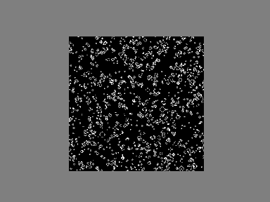
Non-cyclic rendering 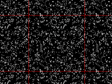
Cyclic rendering
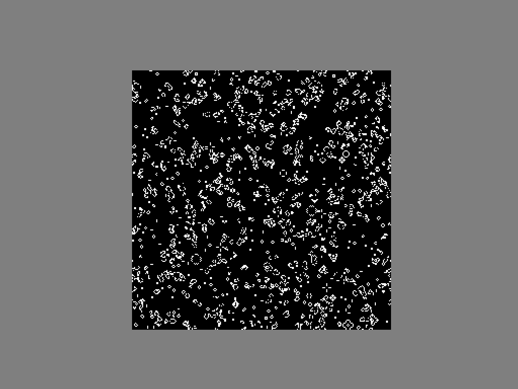
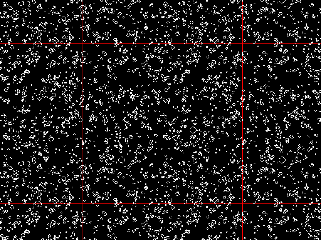
The ability to read both byte-per-cell and bit-per-cell formats of the life world is handy to avoid any unnecessary conversions of data formats. Conversion is handled right in the display kernel with very little overhead.
Zooming is done just by simple multiplication of the coordinates by zoomFactor.
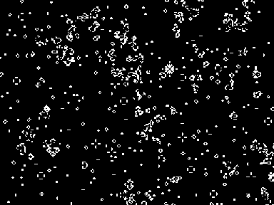
Figure 24 shows zoomed-in, native and zoomed-out screenshots of a life world.
Zoomed in 2× 
Native resolution (pixel per cell) 
Zoomed out 2×
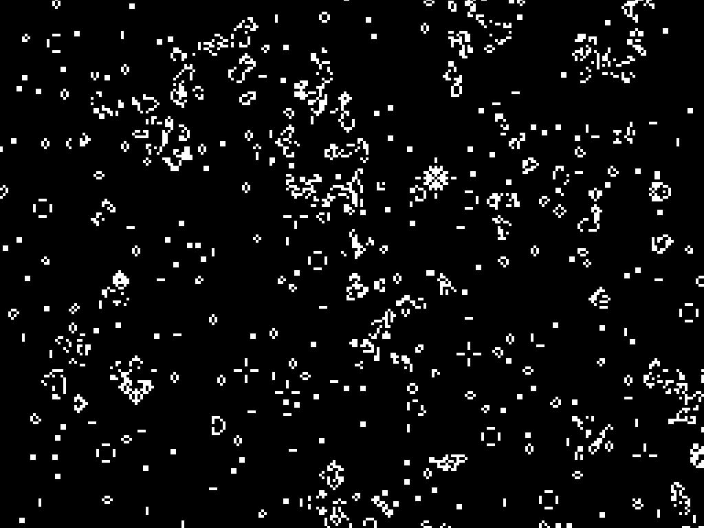

The multi-sampling technique is used to average colors of all life cells in every pixel if the world is zoomed-out.
Drawing of life boundaries is a minor thing but if cyclic rendering is turned on it is impossible to know where world boundaries are. The boundary is rendered cleverly – it does not hide alive cells, it is shown only over dead cells.
1
2
3
4
5
6
7
8
9
10
11
12
13
14
15
16
17
18
19
20
21
22
23
24
25
26
27
28
29
30
31
32
33
34
35
36
37
38
39
40
41
42
43
44
45
46
47
48
49
50
51
52
53
54
__global__ void displayLifeKernel(const ubyte* lifeData, uint worldWidth,
		uint worldHeight, uchar4* destination, int destWidth, int detHeight,
		int2 displacement, double zoomFactor, int multisample,
		bool simulateColors, bool cyclic, bool bitLife) {

	uint pixelId = blockIdx.x * blockDim.x + threadIdx.x;

	int x = (int)floor(((int)(pixelId % destWidth) - displacement.x) * zoomFactor);
	int y = (int)floor(((int)(pixelId / destWidth) - displacement.y) * zoomFactor);

	if (cyclic) {
		x = ((x % (int)worldWidth) + worldWidth) % worldWidth;
		y = ((y % (int)worldHeight) + worldHeight) % worldHeight;
	}
	else if (x < 0 || y < 0 || x >= worldWidth || y >= worldHeight) {
		destination[pixelId].x = 127;
		destination[pixelId].y = 127;
		destination[pixelId].z = 127;
		return;
	}

	int value = 0;  // Start at value - 1.
	int increment = 255 / (multisample * multisample);

	if (bitLife) {
		for (int dy = 0; dy < multisample; ++dy) {
			int yAbs = (y + dy) * worldWidth;
			for (int dx = 0; dx < multisample; ++dx) {
				int xBucket = yAbs + x + dx;
				value += ((lifeData[xBucket >> 3] >> (7 - (xBucket & 0x7))) & 0x1) * increment;
			}
		}
	}
	else {
		for (int dy = 0; dy < multisample; ++dy) {
			int yAbs = (y + dy) * worldWidth;
			for (int dx = 0; dx < multisample; ++dx) {
				value += lifeData[yAbs + (x + dx)] * increment;
			}
		}
	}

	bool isNotOnBoundary = !cyclic || !(x == 0 || y == 0);

	if (simulateColors) {
		// Post-processing is described in next section ...
	}
	else {
		destination[pixelId].x = isNotOnBoundary ? value : 255;
		destination[pixelId].y = value;
		destination[pixelId].z = value;
	}
	destination[pixelId].w = value;
}
Texture post-processing#
Black and white rendering of Conway's Game of Life is classic but I did not like it. Since the CUDA kernel offers full control of assigned colors to each pixel I decided to make it more alive by some simple post-processing.
The alpha channel destination[pixelId].w is used to store the previous cell value.
Based on this information it is possible to distinguish between the following four states:
- was alive and is alive (stayed alive),
- was alive and is dead (died),
- was dead and is dead (stayed dead), and
- was dead and is alive (born).
This information is used to color the cells in the following way:
- every born cell is white,
- every alive cell gets darker over time until it is dark gray, and
- every cell that dies leaves a dark green trace that gets darker over time until it gets black.
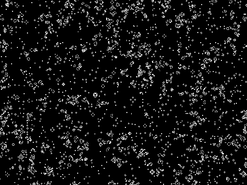
Figure 25 shows those rules written in the CUDA kernel code which is part of Code listing 16. The effect of described post-processing can be seen in Figure 25.
This effect was made just for fun and due to the way previous states are saved; any movement or zoom of the world resets the post-processing.
With post-processing 
Without post-processing
1
2
3
4
5
6
7
8
9
10
11
12
13
14
15
16
17
18
19
20
21
22
23
24
25
26
27
28
29
30
31
32
33
34
35
36
37
38
39
40
41
42
43
44
45
46
	if (simulateColors) {
		if (value > 0) {
			if (destination[pixelId].w > 0) {
				// Stayed alive - get darker.
				if (destination[pixelId].y > 63) {
					if (isNotOnBoundary) {
						--destination[pixelId].x;
					}
					--destination[pixelId].y;
					--destination[pixelId].z;
				}
			}
			else {
				// Born - full white color.
				destination[pixelId].x = 255;
				destination[pixelId].y = 255;
				destination[pixelId].z = 255;
			}
		}
		else {
			if (destination[pixelId].w > 0) {
				// Died - dark green.
				if (isNotOnBoundary) {
					destination[pixelId].x = 0;
				}
				destination[pixelId].y = 128;
				destination[pixelId].z = 0;
			}
			else {
				// Stayed dead - get darker.
				if (destination[pixelId].y > 8) {
					if (isNotOnBoundary) {
					}
					destination[pixelId].y -= 8;
				}
			}
		}
	}
	else {
		destination[pixelId].x = isNotOnBoundary ? value : 255;
		destination[pixelId].y = value;
		destination[pixelId].z = value;
	}

	// Save last state of the cell to the alpha channel that is not used in rendering.
	destination[pixelId].w = value;
Texture drawing#
Finally, Code listing 18 shows actual code for drawing the texture using OpenGL. It is done by drawing a single quadrilateral across the whole screen with correct texture coordinates.
Somebody may criticize the usage of OpenGL fixed pipeline functions for drawing a quad but hey, it's just a single quad. More interesting code is the one that actually writes the information to the texture. This is described in the next section.
1
2
3
4
5
6
7
8
9
10
11
12
13
14
15
16
17
18
19
20
21
22
void drawTexture() {
	glColor3f(1.0f, 1.0f, 1.0f);
	glBindTexture(GL_TEXTURE_2D, gl_texturePtr);
	glBindBuffer(GL_PIXEL_UNPACK_BUFFER_ARB, gl_pixelBufferObject);

	glTexSubImage2D(GL_TEXTURE_2D, 0, 0, 0, screenWidth, screenHeight,
		GL_RGBA, GL_UNSIGNED_BYTE, 0);

	glBegin(GL_QUADS);
	glTexCoord2f(0.0f, 0.0f);
	glVertex2f(0.0f, 0.0f);
	glTexCoord2f(1.0f, 0.0f);
	glVertex2f(float(screenWidth), 0.0f);
	glTexCoord2f(1.0f, 1.0f);
	glVertex2f(float(screenWidth), float(screenHeight));
	glTexCoord2f(0.0f, 1.0f);
	glVertex2f(0.0f, float(screenHeight));
	glEnd();

	glBindBuffer(GL_PIXEL_UNPACK_BUFFER_ARB, 0);
	glBindTexture(GL_TEXTURE_2D, 0);
}
6. Conclusion#
This project presented three different conventional evaluation algorithms for Conway's Game of Life: basic algorithm, bit counting algorithm, and lookup table algorithm. All three algorithms were carefully implemented on both CPU and GPU and a thorough benchmark was performed.
The best algorithm for the CPU turned out to be the lookup table that yields speedups up to 45× over the serial CPU. The best algorithm for the GPU was the bit counting with a speedup of 480× over the serial CPU. The following section shows detailed graphs and a comparison of all algorithms.
Hardware#
CPU: Xeon E5530 @ 2.40GHz with 4 cores (8 threads)
GPU: GeForce GTX 580 with 1.5 GB of graphics memory and 512 CUDA cores
Overall performance evaluation#
Figure 26 presents absolute evaluation speeds in millions of evaluated cells per second. The GPU is able to evaluate an amazing 28 trillion cells per second. This number is hard to imagine. I like to compare fast things with fast things, say with the speed of light – nearly 300,000 km/s, that's 1,000,000,000 km/h (671,000,000 mph).
How far can light travel until one life cell is evaluated (on average)?
The distance per evaluated cell dpc can be computed as:
dpc = c/es = 299,792,458/24,688,686,207 = 0.01214 m, where dpcis distance per evaluated cell in meters,cis speed of light in m/s, andesis evaluation speed in cells/s.
One cell is evaluated for every 0.01214 meters passed by light! That's 12 mm or 0.48 in! That is quite mind-blowing. Let me know if you have any conventional (no hash-life) algorithm that performs significantly better on comparable hardware.
The last two charts present speedup over the serial CPU (Figure 27) and over the parallel CPU (Figure 28). The GPU is reaching speedup of 480× over the serial CPU or 235× over the parallel CPU algorithms. I consider those speedups as satisfying results.
Code and supplementary material#
You can find full source code published under Public Domain on GitHub.
Download
- GameOfLifeCuda-Benchmark.ods — Spreadsheet with all benchmark results and computations used in this article.