April 2013
Real time visualization of 3D vector field with CUDA
4 Vector field integrators for stream line visualization
4.1 Euler integrator
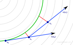
dt = 0.5 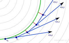
dt = 0.25
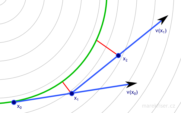

Figure 1: Euler integration for dt = 0.5 and 0.25. Vector field is shown as thin gray lines, green curve represents ground truth, blue arrows are vectors used in computation of Euler's integration, and red lines shows error.
Code listing 1: Euler integrator in CUDA
1 2 3 4 | __device__ double4 eulerIntegrate(double3 pos, double dt) { float4 v = tex3D(vectorFieldTex, (float)pos.x, (float)pos.y, (float)pos.z); return make_double4(dt * v.x, dt * v.y, dt * v.z, v.w); } |
4.2 Runge–Kutta 4 integrator
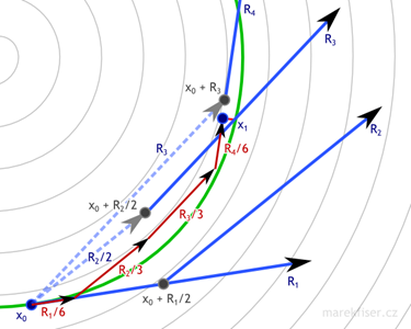
One step or RK4 integration with dt = 1. Vector field is shown as thin gray lines, green curve represents ground truth, blue arrows are vectors used in computation of RK4 integration, dark red arrows are actual RK4 steps, and small bright red line represents error. Note that RK4 has much smaller error than Euler (Figure 1) even for much bigger time step.

Figure 2: One step or RK4 integration with dt = 1. Vector field is shown as thin gray lines, green curve represents ground truth, blue arrows are vectors used in computation of RK4 integration, dark red arrows are actual RK4 steps, and small bright red line represents error. Note that RK4 has much smaller error than Euler (Figure 1) even for much bigger time step.
Code listing 2: Runge–Kutta 4 integrator in CUDA
1 2 3 4 5 6 7 8 9 10 11 12 13 14 15 16 17 18 | __device__ double4 rk4Integrate(double3 pos, double dt) { double dtHalf = dt * 0.5; float4 k1 = tex3D(vectorFieldTex, (float)pos.x, (float)pos.y, (float)pos.z); float4 k2 = tex3D(vectorFieldTex, (float)(pos.x + dtHalf * k1.x), (float)(pos.y + dtHalf * k1.y), (float)(pos.z + dtHalf * k1.z)); float4 k3 = tex3D(vectorFieldTex, (float)(pos.x + dtHalf * k2.x), (float)(pos.y + dtHalf * k2.y), (float)(pos.z + dtHalf * k2.z)); float4 k4 = tex3D(vectorFieldTex, (float)(pos.x + dt * k3.x), (float)(pos.y + dt * k3.y), (float)(pos.z + dt * k3.z)); double dtSixth = dt / 6.0; return make_double4( dtSixth * (k1.x + 2.0 * ((double)k2.x + k3.x) + k4.x), dtSixth * (k1.y + 2.0 * ((double)k2.y + k3.y) + k4.y), dtSixth * (k1.z + 2.0 * ((double)k2.z + k3.z) + k4.z), (k1.w + 2.0 * ((double)k2.w + k3.w) + k4.w) / 6.0); } |